Computer Vision (CV) models use training data to learn the relationship between input and output data. The training is an optimization process. Gradient descent is an optimization method based on a cost function.

Contents
Computer Vision (CV) models use training data to learn the relationship between input and output data. The training is an optimization process. Gradient descent is an optimization method based on a cost function. It defines the difference between the predicted and actual value of data.
CV models try to minimize this loss function or lower the gap between prediction and actual output data. To train a deep learning model – we provide annotated images. In each iteration – GD tries to lower the error and improve the model’s accuracy. Then it goes through a process of trials to achieve the desired target.
Dynamic Neural Networks use optimization methods to arrive at the target. They need an efficient way to get feedback on the success. Optimization algorithms create that feedback loop to help the model accurately hit the target.
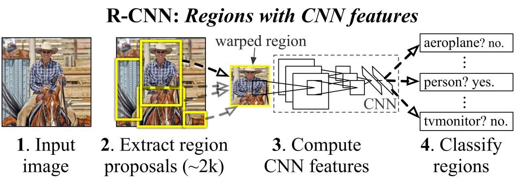
Deep Learning with Convolutional Neural Network
For example, image classification models use the image’s RGB values to produce classes with a confidence score. Training that network is about minimizing a loss function. The value of the loss function provides a measure – of how far from the target performance a network is with a given dataset.
In this article, we elaborate on one of the most popular optimization methods in CV Gradient Descent (GD).
About us: ProX PC is the enterprise machine learning infrastructure that hands complete control of the entire application lifecycle to ML teams. With top-of-the-line security measures, ease of use, scalability, and accuracy, ProX PC provides enterprises with 695% ROI in 3 years. To learn more, book a demo with our team.
What is Gradient Descent?
The best-known optimization method for a function’s minimization is gradient descent. Like most optimization methods, it applies a gradual, iterative approach to solving the problem. The gradient indicates the direction of the fastest ascent. A negative gradient value indicates the direction of the fastest descent.
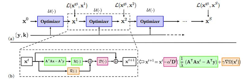
Gradient descent algorithm, y is blurry image, x(t+1)-the new estimate
We can illustrate this with dog training. The training is gradual with positive reinforcements when reaching a particular goal. We start by getting its attention and giving it a treat when it looks at us.
With that reinforcement (that it did the right thing with the treat), the dog will continue to follow your instructions. Therefore – we can reward it as it moves to achieve the desired goal.
How does Gradient Descent Work?
As mentioned above – we can treat or compute the gradient as the slope of a function. It is a set of a function’s partial derivatives concerning all variables. It denotes the steepness of a slope and it points in the direction where the function increases (decreases) fastest.
We can illustrate the gradient – by visualizing a mountain with two peaks and a valley. There is a blind man at one peak, who needs to navigate to the bottom. The person doesn’t know which direction to choose, but he gets some reinforcement in case of a correct path. He moves down and gets reinforcement for each correct step, so he will continue to move down until he reaches the bottom.
Learning Rate is an important parameter in CV optimization. The model’s learning rate determines whether to skip certain parts of the data or adjust from the previous iteration.
In the mountain example this would be the size of each step the person takes down the mountain. In the beginning – he may take large steps. He would descend quickly but may overshoot and go up the other side of the mountain.
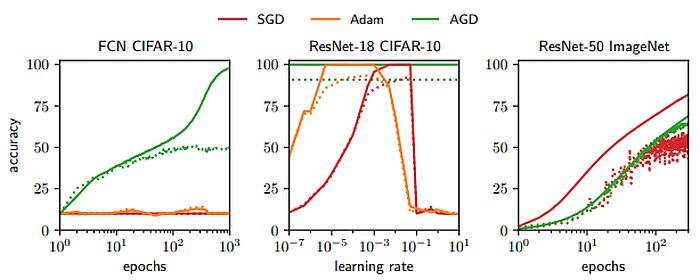
Automatic Gradient Descent trains neural networks
Learning Rate in Gradient Descent
Gradient Descent is an iterative optimization algorithm that finds the local minimum of a function. A lower learning rate is better for real-world applications. It would be ideal if the learning rate decreases as each step goes downhill.
Thus, the person can reach the goal without going back. For this reason, the learning rate should never be too high or too low.
Gradient Descent calculates the next position by using a gradient at the current position. We scale up the current gradient by the learning rate. We subtract the obtained value from the current position (making a step). Learning rate has a strong impact on performance:
Issues with Gradient Descent
Complex structures such as neural networks involve non-linear transformations in the hypothesis function. It’s possible that their loss function doesn’t look like a convex function with a single minimum. The gradient can be zero at a local minimum or zero at a global minimum throughout the entire domain.
If it arrives at the local minima – it will be difficult to escape that point. There are also saddle points, where the function is a minima in one direction and a local maxima in another direction. It gives the illusion of converging to a minimum.
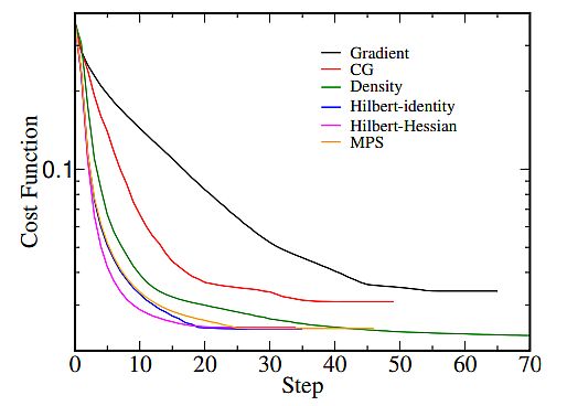
The cost function of different algorithms, including GD
It is important to overcome these gradient descent challenges:
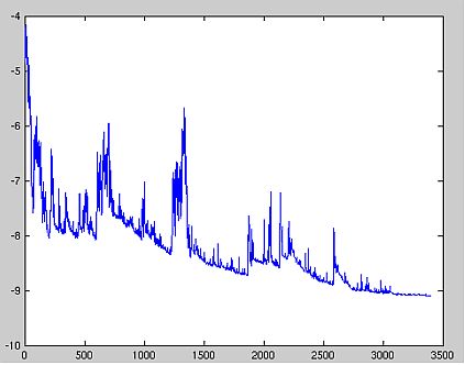
Monitoring the gradient descent on plots will allow you to determine if it’s not working properly – in cases when the cost function is increasing. In most cases, the reason for an increasing cost function when using gradient descent is a large learning rate.
Types of Gradient Descent
Based on the amount of data the algorithm uses – there are 3 types of gradient descent:
Stochastic Gradient Descent
Stochastic gradient descent (SGD) updates the parameters for each training example subsequently. In some scenarios – SGD is faster than the other methods.
An advantage is that frequent updates provide a rather detailed rate of improvement. However – SGD is computationally quite expensive. Also, the frequency of the updates results in noisy gradients, causing the error rate to increase.
Fluctuation of the Stochastic gradient descent
| for i in range (nb_epochs): np. random shuffle (data) for example in data: params_grad evaluate_gradient (loss_function, example, params) params params learning_rate params_grad |
Batch Gradient Descent
Batch gradient descent uses recurrent training epochs to calculate the error for each example within the training dataset. It is computationally efficient – it has a stable error gradient and a stable convergence. A drawback is that the stable error gradient can converge in a spot that isn’t the best the model can achieve. It also requires loading of the whole training set in the memory.
| for i in range (nb_epochs): params_grad = evaluate_gradient (loss_function, data, params) params = params - learning_rate * params_grad |
Gradient Descent and Mini-Batch
Mini-batch gradient descent is a combination of the SGD and BGD algorithms. It divides the training dataset into small batches and updates each of these batches. This combines the efficiency of BGD and the robustness of SGD.
Typical mini-batch sizes range around 100, but they may vary for different applications. It is the preferred algorithm for training a neural network and the most common GD type in deep learning.
| for i in range (nb_epochs): np.random . shuffle (data) for batch in get_batches (data , batch_size =50): params_grad = evaluate_gradient (loss_function, batch, params ) params = params - learning_rate * params_grad |
What’s Next?
Developers don’t interact with gradient descent algorithms directly. Model libraries like TensorFlow, and PyTorch, already implement the gradient descent algorithm. But it is helpful to understand the concepts and how they work.
The CV platforms can simplify this aspect for developers even further. They don’t have to deal with a bunch of code. They can quickly annotate the data and focus on the real value of their application. CV platforms reduce the complexity of computer vision and perform many of the manual steps that are difficult and time-consuming.
For more info visit www.proxpc.com
Related Products
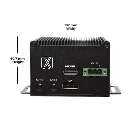
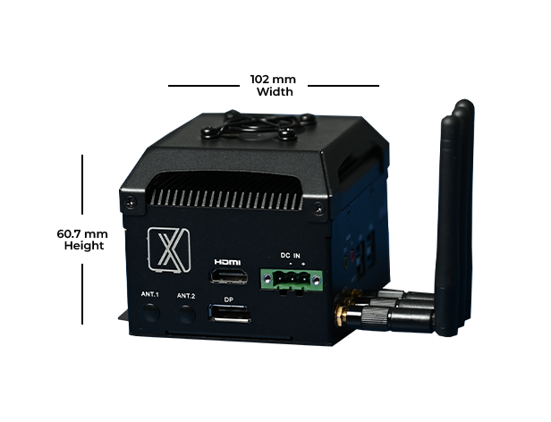
Resources you may find helpful.

The evolution of computer vision technology has paved the way for innovative artificial intelligence (AI).
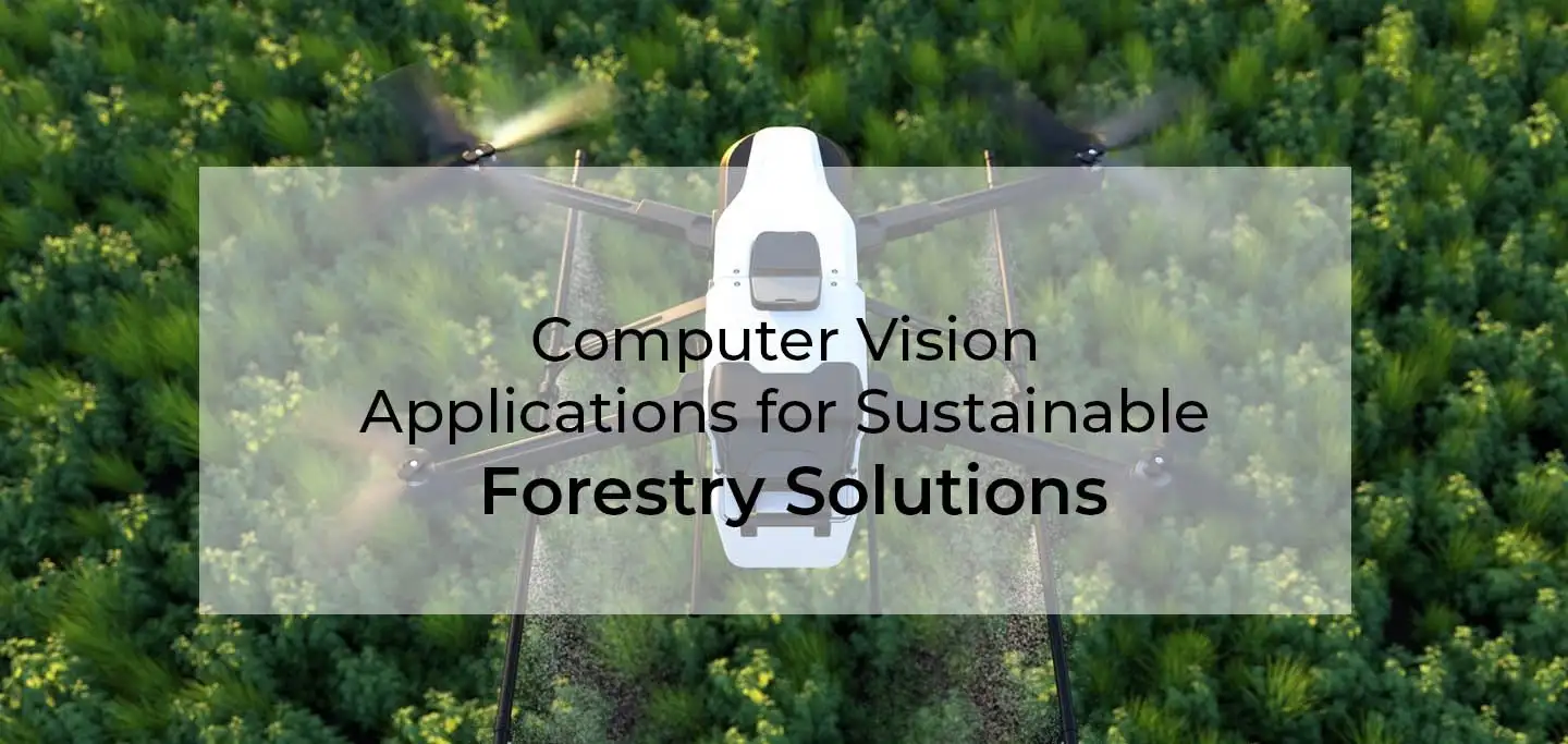
In the past centuries, we saw an increase in deforestation activities such as cutting down trees for wood, extraction of natural resources.

Today's conservation efforts face several challenges that lay the foundation for the need for computer vision and Artificial Intelligence (AI)

The integration of Artificial Intelligence (AI) technologies within the finance industry has fully transitioned from experimental to indispensable.
